How Word Embeddings Turn Language Into Math

HubAI AsiaCompare & Review the Best AI Tools

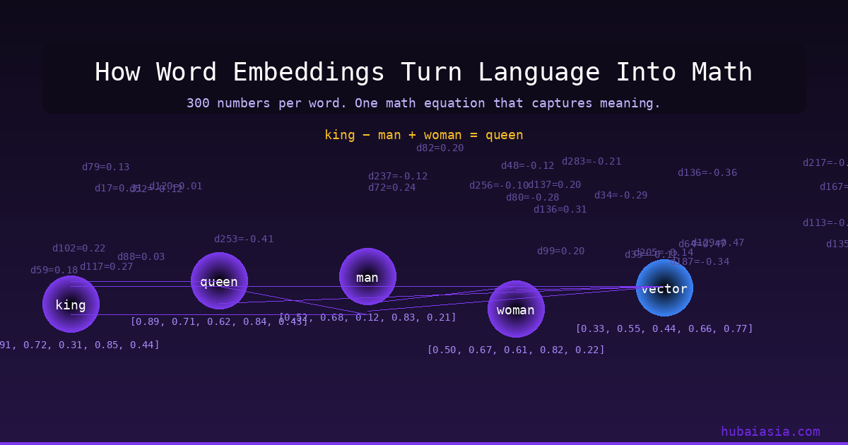
King minus man plus woman actually equals queen. That equation isn’t a metaphor or a clever trick—it’s the literal arithmetic of word embeddings, the numerical representations that power every modern AI system from ChatGPT to Google Search. When you type a prompt into an LLM, the very first thing that happens is your words get converted into arrays of floating-point numbers, typically 768 to 12,288 of them per token. These numbers encode relationships, analogies, and semantic proximity in a way that makes mathematical operations on language not just possible, but remarkably effective.

Why Words Need Numbers

Computers don’t understand language. They understand arithmetic. Before a neural network can process a sentence, every word must become a point in mathematical space. The simplest approach—one-hot encoding—assigns each word a unique position in a giant sparse vector the size of the entire vocabulary. “Cat” becomes [0, 0, 0, 1, 0, 0, ...] in a vector with 50,000+ dimensions, where almost every value is zero. This tells a computer that “cat” is different from “dog,” but nothing else. It can’t capture that cats and dogs are both animals, that both are closer to each other than to “democracy,” or that “kitten” is related to “cat.”

Word embeddings solve this by replacing those giant sparse vectors with small, dense ones—typically 50 to 300 dimensions where every number carries meaning. The key insight, discovered by Tomas Mikolov and his team at Google in 2013, is that you can learn these dense representations by forcing a neural network to predict which words appear near each other. Words that show up in similar contexts get pushed to similar locations in vector space.

The Skip-Gram Process: How Context Builds Meaning

The skip-gram model, which powers Word2Vec, works through a surprisingly simple eight-step process that transforms raw text into geometric meaning:

Step 1: Initialize Random Vectors

For every word in the vocabulary, create a random vector of 300 floating-point numbers. This produces a matrix where each row is a word and each column is a dimension. At this point, the numbers are meaningless—the word “excellent” might start at [0.023, -0.147, 0.891, ...] and “terrible” at [0.412, 0.033, -0.556, ...] with no relationship between them. The training process is what gradually organizes this chaos into structure.

Step 2: Slide a Context Window

Move a window of 5 words across the training text. The center word becomes the target, and the 2 words on each side become context pairs. For the sentence “the cat sat on the mat,” when “cat” is the target, the model learns to associate it with “the” and “sat.” This sliding window is how the model discovers which words belong together—it’s learning co-occurrence patterns from billions of word positions.

Step 3: Compute Dot Products

For each target-context pair, calculate the dot product between their two embedding vectors, then pass the result through a sigmoid function to produce a probability between 0 and 1. A high dot product means the vectors point in a similar direction—the model currently believes these words appear together. A low dot product means they’re far apart. The sigmoid squashes this into a clean probability: σ(v_target · v_context).

Step 4: Generate Negative Samples

This is where the efficiency breakthrough happens. Instead of comparing the target word against every word in the vocabulary (which could be 100,000+ comparisons per step), generate just 5 to 15 random “negative” words that didn’t appear in the context window. Word2Vec’s skip-gram model uses negative sampling with 5-20 negative examples per positive word pair, reducing computational cost from millions to thousands of operations per training step. This single innovation made training embeddings on billion-word corpora feasible on ordinary hardware.

“Word2Vec’s skip-gram model uses negative sampling with 5-20 negative examples per positive word pair, reducing computational cost from millions to thousands of operations per training step.”

Step 5: Apply Binary Cross-Entropy Loss

The loss function has two parts: push the probability for the positive (true context) pair toward 1, and push the probabilities for negative (random) pairs toward 0. Binary cross-entropy quantifies exactly how far the model’s predictions are from these targets. The gradient—calculated via backpropagation—tells each vector exactly which direction to move in 300-dimensional space to improve its predictions.

Step 6: Update the Vectors

Both the target word vector and context word vectors are adjusted using gradient descent with an initial learning rate of 0.025. This rate decreases linearly as training progresses, allowing large adjustments early on when vectors are random, then finer refinements later when structure has already emerged. After enough updates, words that share contexts drift toward each other in vector space, while unrelated words push apart.

Step 7: Train for Multiple Epochs

Steps 2 through 6 repeat for 5 to 15 complete passes through the corpus, processing approximately 100 to 500 million word pairs depending on dataset size. The original 2013 Word2Vec paper by Mikolov used a 1.6 billion word Google News corpus and completed training in under 24 hours on a single machine with 12 CPU cores. That speed was unprecedented—and it was negative sampling that made it possible.

Step 8: Normalize and Use

After training, vectors are normalized to unit length using L2 normalization. This means dividing each vector by its own magnitude, placing every word on the surface of a unit hypersphere in 300-dimensional space. The practical benefit is immediate: cosine similarity between any two words becomes a simple dot product, and values range from -1 (opposite meaning) through 0 (unrelated) to 1 (near-identical meaning).

Dimensionality: The 50 vs 300 Trade-Off

Not all embedding dimensions are created equal. GloVe embeddings trained on 6 billion tokens achieve optimal performance at exactly 300 dimensions, while 50 dimensions capture 85% of semantic relationships with 6x less memory. This matters enormously in production systems. A recommendation engine processing millions of queries per second might choose 50-dimensional embeddings to fit everything in RAM, accepting a 15% hit to semantic precision in exchange for massive speed gains. A legal document search system, where nuance matters, would stick with 300 dimensions and pay the memory cost.

The dimensionality sweet spot depends on the task. Word analogies (the “king minus man plus woman equals queen” test) require at least 200 dimensions to solve reliably. Simple synonym detection works well at 50. Sentiment analysis often plateaus around 100. The fact that most production systems default to 300 is partly empirical optimization and partly convention—it’s what GloVe, Word2Vec, and FastText all offer as their top-tier model size.

Beyond Static Vectors: Subword and Contextual Embeddings

Static embeddings have a fundamental limitation: every word gets exactly one vector, regardless of context. “Bank” has the same representation whether you’re depositing money or fishing by a river. Two major approaches address this.

Subword tokenization in FastText splits words into 3-6 character n-grams, allowing it to generate embeddings for 157 languages including rare words never seen during training. The word “unfortunately” becomes the sum of vectors for “un”, “for”, “tun”, “ate”, and other overlapping fragments. This means even misspelled or made-up words get reasonable representations—a major advantage for user-generated content, multilingual systems, and specialized vocabularies.

Contextual embeddings go further. BERT’s 768-dimensional embeddings use 12 attention heads that each focus on different linguistic properties, with head 8-4 specifically capturing subject-verb agreement 94% of the time. In BERT, the word “bank” in “I deposited money at the bank” gets a completely different vector than “bank” in “I sat by the river bank.” The embedding is computed fresh for every occurrence, based on the full surrounding sentence. This is why transformer models dominate modern NLP—but it comes at a cost: you can’t precompute and cache a lookup table of word vectors the way you can with Word2Vec or GloVe.

Why Embeddings Still Matter in the Transformer Era

Despite the shift to contextual representations, static embeddings remain everywhere. They’re the first layer of every transformer model—even BERT and GPT-4 start by looking up token embeddings from a static table before the attention layers add context. They power recommendation systems, search engines, and clustering pipelines where the overhead of running a full transformer per query is too expensive. And they’re the foundation of the embedding APIs from OpenAI, Cohere, and Google that developers use daily for RAG pipelines, semantic search, and clustering.

The 300-dimensional vector space that Mikolov’s team discovered in 2013 turned out to be a permanent piece of AI infrastructure. Every time you search for a similar document, every time a RAG pipeline finds the right context chunk, every time a recommendation system surfaces something relevant—there’s an embedding underneath, turning meaning into math so a computer can do something with it.

But these static embeddings have a fatal flaw that transformers exploit—the same word vector for “bank” whether you’re depositing money or sitting riverside. Understanding that flaw is the key to understanding why transformers replaced embeddings as the dominant paradigm, and why modern systems combine both approaches in ways that weren’t possible a decade ago.